Tweet Sentiment Extraction

Introduction

Understanding what descriptions lead to certain sentiment in language is important nowadays when reactions to various decisions are made in seconds on social media. The goal of this project is to construct a model for a given sentence and the label sentiment to predict what phrases in the sentence that best support the given sentiment. In natural language processing, we can formulate this task as a question-answering task where sentiment is a question, the tweet is the context, and the support phrase is the answer. We compare several popular neural network models such as the Long-short Term Memory (LSTM), Gated Recurrent Unit (GRU) for this task. Under a word similarity metric, Jaccard score, we are able to achieve 0.607 score with the model.

Methods and Results

Exploratory Data Analysis and Processing

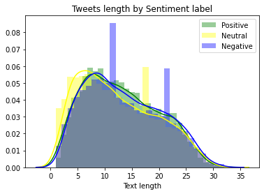
Prior to model building, it is always good to explore the dataset first. From the distribution of the sentiment in the tweets, we can see that tweets that carry netrual sentiment tend to be shorter than those that are positive or negative. We also see that negative sentiment frequently occurs at text length around 10 or 20. The collected tweets hardly go over 35 words.

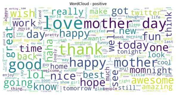
Next, we can get a sense of what words that contribute to different sentiments in the tweets. We plot three different wordclouds to show different collections of vocabularies that count towards different types of sentiment. For the positive wordcloud, the main words include “love”, “thank”, “good”.

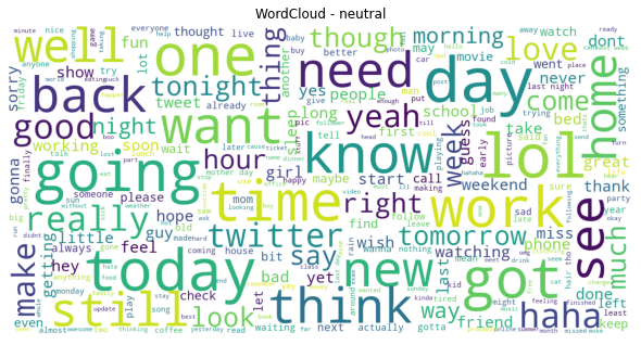
Interestingly, as we look at the neutral word cloud, we see that the main words include “today”, “going”, “want”, “need”.

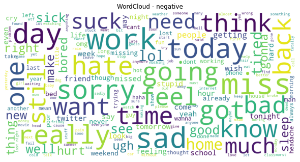
Then, we can see from the negative word cloud that people mostly express their negative sentiment through words like “really”, “sad”, “sorry”.

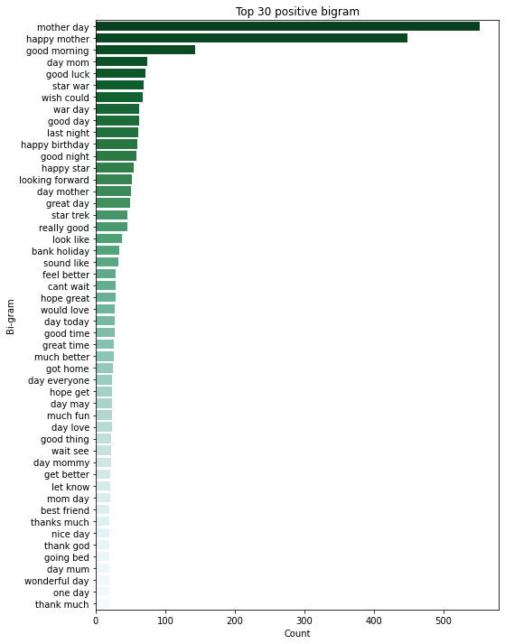
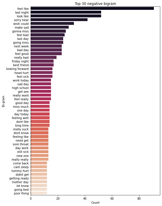
Besides, we can look at two words together at a time, which is known as bigram, to understand which two words go together often in different sentimental tweets. We can see that “mother day” and “happy mother” are strongly associated with positive sentiment. In addition, negative sentiment is mostly associated with “feel like” and “last night”. It maybe good to look into those tweets with “last night” to see if most of them come from news.

Evaluation Metric

The metric in this project is the word-level Jaccard score as follows:

where A, B are sets of words, and |.| denotes the cardinality.

Bidirectional LSTM and GRU with word embedding

The first two neural network architectures we use learn to predict a binary sequence to find the positions corresponding to the selected text inside a given sentence. It consists of the following components: a bidirectional LSTM layer (interchangeable with a GRU layer to become a bidirectional GRU (B-GRU)), a dropout layer, a fully connected layer, a dropout layer, a fully connected layer, a dropout layer, and an output layer. Time distributed layer is added in between droput, full-connected layer, and the output layer.

We use the Keras API in Tensorflow to build a model that consist of the following components in order:

1. Input layer with maximum list length among all the sentences in text column in the data. It can be incorporated in the bidirectional layer argument.

2. A bidirectional LSTM/GRU layer with 20 units, set return sequence = True, dropout=0.3, recurrent dropout = 0.3.

3. A dropout layer with 0.5 rate followed by a fully connected layer with 64 units and set kernel constraint=max norm(3). When use LSTM layer, change the activation in the first layer to be “relu” and the second activation to be “tanh”. When using GRU, the first activation should be “tanh” and the second activation to be “relu”.

4. Repeat the same set up in 4.

5. A dropout layer with 0.5 rate followed by a one unit output layer with sigmoid activation, which is for binary classification.

Lastly, set the loss function to be binary cross entropy and use SGD(lr=0.1 , momentum=0.9) as the optimizer with accuracy as the metric for compiling model. Then, fit the model with training data and validate on the test set with 32 batch size, 60 epochs. At the end, find all the text from the test set that corresponds 1’s in the predicted vector by using tokenizer to output the corresponding text and compute the Jaccard score.

Implementation Summary

1. Replace any word in the text with <token> if it matches the selected text and create a new column in the dataframe called tokenized text.

2. Use Tokenizer() from tensorflow package to tokenize all sentences in text and tokenized text columns. Specify the parameter Tokenizer(Filter=“”) so it will recognize <token> as a word.

3. Ensure all the words that contain <token> in the tokenizer have the same index in the tokenizer. Then, get the length of the list that contains the longest text in the text column. We then convert each row in text to a list of integers by the indicies in tokenizer and pad all lists to have the same length by the max length we obtained previously with zero, call it X. We also convert the text in tokenized text in the same manner, call it y.

4. For every word in each text in y, if it doesn’t correspond to the index of <token>, we set it to be 0 and 1 otherwise.

5. Then, we randomly shuffle and split X and y with 20% test set for testing the model.

6. Use np.array(X_train).reshape(X_train.shape[0], X_train.shape[1],1).astype(np.float32) to transform the dimension for the training samples and np.array(y_train).reshape(y_train.shape[0], y_train.shape[1],1) to transform the dimension for the response in order to have the model to output a sequence.

Justification for Parameters Use

As recommended by Srivastava et al., 2014, we set a large learning rate and high momentum for the SGD along with dropout and follow a similar fashion to set the kernel_constraint on the weights for each hidden layer, ensuring that the maximum norm of the weights does not exceed a value of 2 . Also, we set 60 epochs as we see the training and validation loss don’t change much after 60 epochs. The increases in learning rate is also recommended by (Srivastava et al., 2014) while using dropout. We set the recurrent dropout in the LSTM/GRU layer as suggested by Gal & Ghahramani, 2016 to use with regular dropout. Setting 0.5 rate is via a process of trial and error.

We tuned various activation functions (tanh, ReLU, sigmoid) for two hidden layers with 20 units and initialized LSTM/GRU with 20 units. Then, after selected a desirable combination of activation functions, we tuned the number of nodes for the LSTM, GRU, and those two hideen layers with 30 and 64 units. We also compare the model performance with and without GloVe embedding for both GRU and LSTM models. Also, we have tried using the default Adam optimizer in keras, but the model has suffered from overfitting. However, we don’t see much improvement by increasing the number of nodes, we decide to use 20 number of unit for computational advantages.

Result and Conclusion

Both the B-LSTM and B-GRU achieve 0.607 Jaccard score. GRU and LSTM perform the same on this task based on our tuned parameters. The process of tuning parameters for neural network model is extremly time-consuming especially when the data dimension is large. For the LSTM and GRU model, we first attempted to try different optimizers, then different number of units for hidden layers, activation functions and number of layers. There are a lot of modification to our codes since we attempt to build a better model. We have also tried using pretained embedding layer such as GloVe, but it was too expensive to train, given the dimension of the embedding and we may have to retune all the parameters. In addition, we use a tokenizer to convert text signal for the LSTM/GRU architecture, however, it may lose the information of the context of the sentence and maybe that’s one of the reasons why BERT seems to perform better than LSTM or GRU for this task.

Data Source

Tweet Sentiment Extraction

Reference

• Kaggle:tweet sentiment extraction. https://www.kaggle.com/c/ tweet-sentiment-extraction.

• Cho, K., Van Merrienboer, B., Bahdanau, D., and Bengio, Y.¨ On the properties of neural machine translation: Encoderdecoder approaches. arXiv preprint arXiv:1409.1259, 2014.

• Chung, J., Gulcehre, C., Cho, K., and Bengio, Y. Empirical evaluation of gated recurrent neural networks on sequence modeling. arXiv preprint arXiv:1412.3555, 2014.

• Devlin, J., Chang, M.-W., Lee, K., and Toutanova, K. Bert: Pre-training of deep bidirectional transformers for language understanding. arXiv preprint arXiv:1810.04805v2, 2018.

• Gal, Y. and Ghahramani, Z. A theoretically grounded application of dropout in recurrent neural networks. In Advances in neural information processing systems, pp. 1019–1027, 2016.

• Hochreiter, S. and Schmidhuber, J. Long short-term memory. Neural computation, 9(8):1735–1780, 1997.

• Srivastava, N., Hinton, G., Krizhevsky, A., Sutskever, I., and Salakhutdinov, R. Dropout: a simple way to prevent neural networks from overfitting. The journal of machine learning research, 15(1):1929–1958, 2014.